MNIST Dataset
This dataset contains 28x28 grayscale images of digits from 0 to 9. In the train csv file, there are 42000 examples/images.
In [1]:
%load_ext autoreload
%autoreload 2
%matplotlib inline
In [2]:
from fastai.vision import Path

path_d = Path("../input/")
path_d.ls()
Out[2]:
In [3]:
import pandas as pd
import numpy as np
import matplotlib.pyplot as plt

df_mnist = pd.read_csv(path_d/"train.csv")
label = np.array(df_mnist["label"])
imgs = np.array(df_mnist.drop(['label'],axis=1))
df_mnist.head(2)
Out[3]:
This function allows us to print out shapes of arrays
In [4]:
def shapes(*x):
    for idx, item in enumerate(x): print(f"arg_{idx}: {item.shape}")
In [5]:
shapes(imgs, label)
Visualize the images in MNIST
In [6]:
from IPython.display import clear_output
import time

dim = int(imgs.shape[1]**0.5)
for i in np.random.permutation(len(imgs))[:10]:
    plt.imshow(imgs[i].reshape(dim,dim)/255,'gray')
    plt.title(label[i])
    plt.show()
    time.sleep(0.1)
    clear_output(wait=True)

This is just to clear RAM so that the kernel does not crash
In [7]:
import gc
del df_mnist, label, imgs
gc.collect()
Out[7]:
This refactor some code to get the MNIST dataset, so that next time, we can call getMNIST() to get the dataset
In [8]:
def scale(x): return x/255
def split_vals(x,y,n): idxs = np.random.permutation(len(x)); return x[idxs[:n]], x[idxs[n:]], y[idxs[:n]], y[idxs[n:]]

def loadMNIST(path_d):
    df_mnist = pd.read_csv(path_d/"train.csv")
    label = np.array(df_mnist["label"])
    imgs = np.array(df_mnist.drop(['label'],axis=1))
    return imgs, label

def getMNIST():
    imgs, label = loadMNIST(Path("../input/"))
    split_amt= round(imgs.shape[0] * 0.90)
    x_train, x_test, y_train, y_test = split_vals(scale(imgs), label, split_amt)
    return x_train, x_test, y_train, y_test
Single Layer Perceptron
In [9]:
x_train, x_test, y_train, y_test = getMNIST()
shapes(x_train, x_test, y_train, y_test)
In [10]:
import tensorflow as tf
from tensorflow import keras

slp_model = keras.Sequential([
    keras.layers.Dense(512, activation=tf.nn.relu, input_shape=([784])),
    keras.layers.Dense(10, activation=tf.nn.softmax)
])

slp_model.compile(optimizer='adam',
              loss='sparse_categorical_crossentropy',
              metrics=['accuracy'])
Classification Loss Functions
- categorical_crossentropy -> classification with one-hot encoded labels (ie. [0,0,1])
- sparse_categorical_crossentropy -> classification with discrete labels (ie. [2])
In [11]:
slp_model.summary()
In [12]:
slp_model.fit(x_train, y_train,
              validation_data=(x_test, y_test),
              epochs=5)
Out[12]:
In [13]:
def softmax(x): return np.exp(x.squeeze())/sum(np.exp(x.squeeze()))
In [14]:
output = np.array([60,50,10,20,40,20,40,50])
softmax(output)
Out[14]:
Lets define a function to visualize our results
In [15]:
def seeResults(model, x, y):
    dim=28
    plt.figure(figsize=(20,20))
    idxs = np.random.permutation(len(x))
    for i,idx in enumerate(idxs[:25]):
        plt.subplot(5,5,i+1)
        plt.xticks([]), plt.yticks([])
        plt.grid(False)
        plt.imshow(x[idx].reshape(dim,dim),'gray')
        pred = softmax(model.predict(x[idx][None,:])) #Here the model makes a prediction
        plt.xlabel(f"Label:{y[idx]}, Pred:{np.argmax(pred)}")
    plt.show()
In [16]:
seeResults(slp_model, x_test, y_test)

In [17]:
??keras.layers.Dense.call
What is matmal() (or dot())

In [18]:
def matmul1(a,b):
    ar,ac = a.shape
    br,bc = b.shape
    assert ac==br
    c = np.zeros(shape=(ar, bc))
    for i in range(ar):
        for j in range(bc):
            for k in range(ac): # or br
                c[i,j] += a[i,k] * b[k,j]
    return c

def matmul2(a,b):
    ar,ac = a.shape
    br,bc = b.shape
    assert ac==br
    c = np.zeros(shape=(ar, bc))
    for i in range(ar):
        for j in range(bc):
            c[i,j] = (a[i,:] * b[:,j]).sum()
    return c

def matmul3(a,b): return np.einsum('ik,kj->ij', a, b)
In [19]:
np.random.seed(0)
a = np.random.randn(128,128)
b = np.random.randn(128,128)

%time x = matmul1(a,b)
%time y = matmul2(a,b)
%time z = matmul3(a,b)
%time t = tf.matmul(a,b)
Lets compare the results, and see if they are really equal
In [20]:
def compare(x,y): print(np.isclose(x,y).all())
compare(x,y), compare(x,z)
Out[20]:
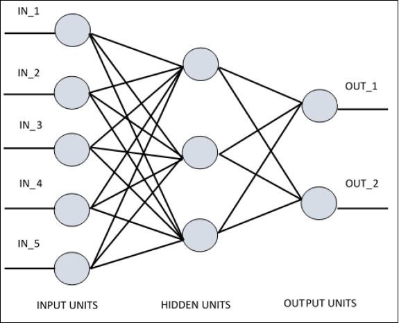
Multi-Layer Perceptron
In [21]:
x_train, x_test, y_train, y_test = getMNIST()
In [22]:
mlp_model = keras.Sequential([
    keras.layers.Dense(512, activation=tf.nn.relu),
    keras.layers.Dense(256, activation=tf.nn.relu),
    keras.layers.Dense(128, activation=tf.nn.relu),
    keras.layers.Dense(10, activation=tf.nn.softmax)
])

mlp_model.compile(optimizer='adam',
              loss='sparse_categorical_crossentropy',
              metrics=['accuracy'])
In [23]:
mlp_model.fit(x_train, y_train, validation_data=(x_test, y_test), epochs=1)
Out[23]:
In [24]:
seeResults(mlp_model, x_test, y_test)
